Warren Buffett has said that trying to time the market is the number one mistake to avoid.

Market timing is hard, if not impossible to do, as it often results in the investor buying or selling too late or too early rather than right on time.  To even consider a market timing strategy is generally frowned upon by professional investors.

But we’re not professional investors, we’re just engineers who were convinced that there must be a simple yet effective way to pick up on and follow trends in uncorrelated asset classes.  We don’t hope or expect to be right every time, but we do hope and expect this strategy to do a decent job at minimizing losses to improve the effect of compounding gains.

In this post, I will lay out the framework of a simple, intuitive and profitable strategy that has worked well over the last 150 years.  I will provide all the data used so that you can perform your own analysis.  I’ll also provide tools you can use to implement this, or a similar strategy, on your own for free.  No proprietary software necessary, no expensive financial advisor required – just you, some logic, and systematic rules-based investing (no emotion!).

---

Table of Contents

This post got a bit out of hand… over 5,000 words.  So here’s a table of contents to let you traverse this a bit better.

• Overview
• Background
• Concerns
• Show Me More Data
• How to Live Trade

Overview

The Rules

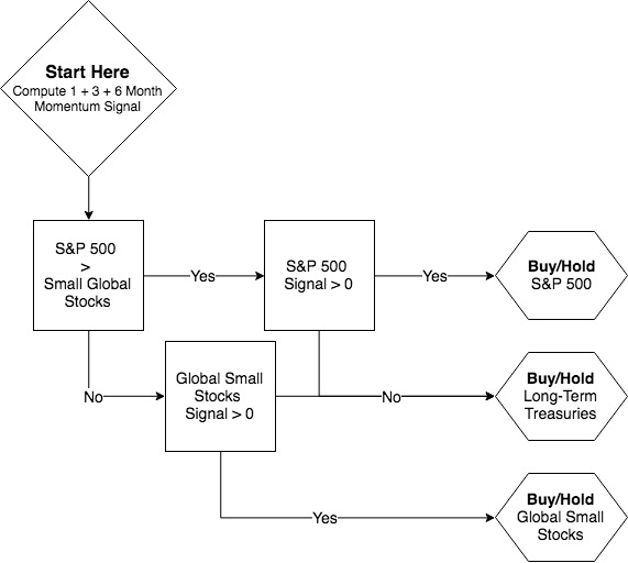
The rules are quite simple.  Compute an accelerating momentum score of US and international stocks, specifically small-cap ex-US stocks for the added correlation benefit.  This momentum score is the sum of each asset’s 1 month, 3-month, and 6-month returns.  Doing the sum of these three time segments lets us also take into account the curve of the trend.  If both scores are below zero, that’s bad and an indicator of a consistent downward trend in stocks – buy bonds (specifically long-term treasuries, again for the added correlation benefit).  Otherwise, buy the asset with the higher momentum trend.  Do this selection at the beginning of every month.

The Results

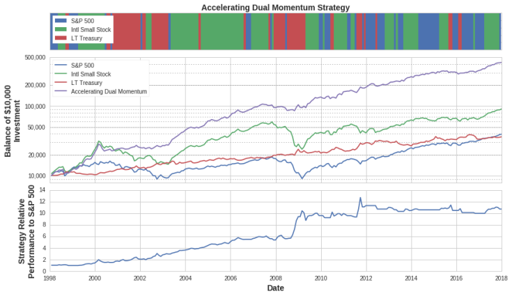
This relatively simple strategy has performed remarkably well over the last 20 years. Because it’s so simple, the strategy can be backtested and explored with Portfolio Visualizer and mutual fund data going back to 1998.  Implementing this strategy with a $10,000 initial investment in 1998 would have grown to over $420,000 by the end of 2017 vs just under $40,000 if invested in the S&P 500 in that time.

Strategy Background

Gary Antonacci’s Dual Momentum

This ex-trader Gary Antonacci wrote a book called “Dual Momentum Investing” where he detailed a strategy that looks at the trailing 12-month return between US stocks and global stocks.  He buys whichever is greater between the two so long as the US trend is positive (even if global stocks are up but the US is down, he’s in bonds) otherwise the strategy says buy bonds.  So you can clearly see the parallels with the strategy I’m laying out here.  Before I get into why I don’t like this implementation, let’s touch on what I do like.

• Simple – only three options, pretty straightforward rules
• Dual momentum – I’ll really like pairing US and global stocks first in a relative momentum signal, then if they’re both negative against an absolute metric to buy bonds.
• Few transactions – in 20 years there are only 23 transactions

Here’s what I don’t like about the strategy.

• 1 year is too long – looking at 1-year returns has the benefit of holding power and minimizing “whipsawing” where the trend signal is constantly changing.  But this also has the consequence of being too late to the party, by the time the signal may pick up a trend it’s already stopped and potentially reversing.
• No measure of consistency – I want to buy the asset that is swinging or accelerating up relative to the others and has some holding power to it.
• Muted diversification benefits – our historical analysis shows that US large cap stocks are becoming increasingly correlated with global large cap (they are all multinational global conglomerates now) so pairing these two against each other may miss the underlying trend and fundamentals.  Same goes for bonds, a total bond fund contains a lot of corporate bonds which are more correlated to stock performance than treasury bonds.  The duration also matters where an intermediate bond fund doesn’t swing as hard, which we actually want in this strategy.

Still, I need to give Gary credit for his research and publishing of his strategy.  I like the dual momentum idea (combining a relative signal with an absolute one).  I recently read the book before publishing this post (wanted to make sure I wasn’t missing anything obvious!) and will say that the book is a good read and reinforces the general premise of why momentum has been effective.

Accelerating Dual Momentum

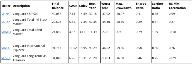
Before we take a look at the strategy’s evolution, let’s first review some metrics of the asset classes we’ll consider during the time period of 1998 to February 2018.  The final balance shown is for an initial investment of $10,000.

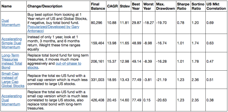
Now let’s take the “original” dual momentum strategy and make some tweaks.  The links are to the individual backtests in Portfolio Visualizer, final balances shown are for a $10,000 investment at the beginning of 1998 growing until February 2018.

• $80,296 – Original Strategy
• $159,464 – Simple Accelerating Dual Momentum
  • Same assets as original but use 1-month, 3-month, and 6-month returns
• $206,161 – Replace Total Bond with Long-Term Treasuries
• $331,003 – Replace Global Large Cap with Global Small Cap
• $426,408 – Accelerating Dual Momentum
  • Make both replacements above, global small cap and long-term treasuries

The following table provides more performance metrics of this strategy and its permutations.  One of the most telling metrics is the reduction in the maximum drawdown of all the strategies (roughly a 20% loss) compared to a buy-and-hold of the S&P 500 (near 60% loss).  Our “Accelerating Dual Momentum” (ADM) strategy has never, historically, had a year with a loss (certainly not a guarantee moving forward).

Accelerating Momentum Signal

One of the major elements of this strategy is how it looks to find consistent uptrends that are accelerating upward.  Here’s a real example from April of 2017.  Over the preceding 6 months, US large-cap stocks had beaten small cap international stocks by a little over 5%.  But over the last 3 months, small-cap global stocks had a 9% gain vs a 6% for the US.  And in the most recent month, small-cap global continued to advance with a 2% gain while the US fell 1%.

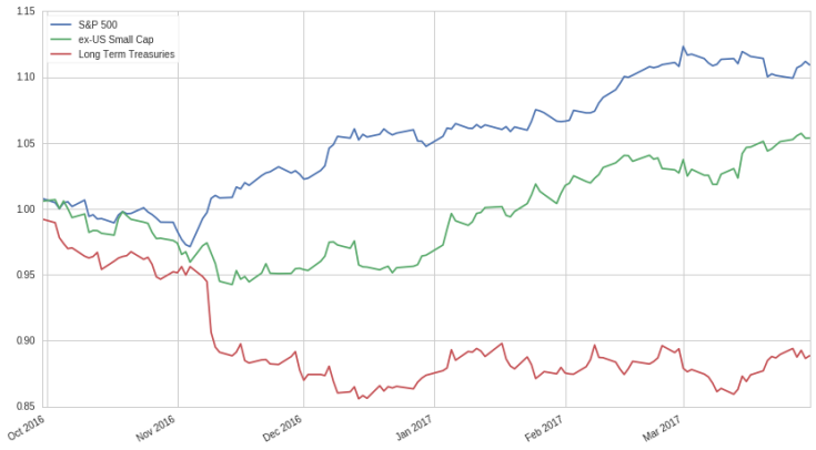
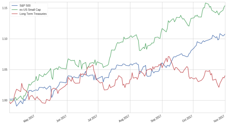
Because our scoring doesn’t just look solely at the trailing 6-month performance but also takes into consideration the other more recent time periods we would weight small-cap international stocks higher.  In the following 8 months after this decision point, the strategy would have stayed with small-cap global stocks which outperformed US large cap by 5%.  But towards the end of this period, it now began appearing that US stocks had the more consistent gains performance and so it switches back to the US.

Tracking Error

When analyzing different potential investment strategies many, including myself, can get caught up in looking at the final number the investment grew to – it doesn’t tell the story it took to get there.  And investors need to not only be able to tolerate the volatility of absolute returns, they need to tolerate the volatility of returns relative to the benchmark.

“Tracking error” looks to quantify how a strategy does relative to a benchmark, the higher the “error” the less correlated it is to the benchmark, which is often the S&P 500.

If you’re trying to beat the benchmark you will undoubtedly lose to it every now and then (because you’ll be different than it) with the hope that it will more frequently beat it.  The question is, how long can you stand to continue to lose to the benchmark before you abandon the strategy (which may be at the absolute worst time, right when it’s about to be effective)?

Value stocks are a good example.  They have been shown to historically outperform growth, but that outperformance requires the investor to endure extended stretches of time (months, even years) when it underperforms the general market (2017 prime example).  And it can be very difficult to keep your conviction when you’re losing to a free alternative which would be an S&P 500 index fund.

The importance of tracking error will matter differently depending on the person and the strategy.  As Chris suggests in his post on combating your cave man brain – you may be better off checking your account frequently.  I agree with him, I’ve learned quite a lot by seeing what’s going on more frequently.  The trouble is… tracking error is a bigger deal if you are checking your account more often.  If you are interested in the static “engineered portfolios” then you likely can live with checking your account on a quarterly or even yearly basis – in which case tracking error will matter less.  But if you are reading this blog and interested in a monthly switching strategy… by definition you will be checking your account more frequently and tracking error will be a greater concern.

So how does this strategy do relative to the benchmark, the S&P 500? Unusually well.

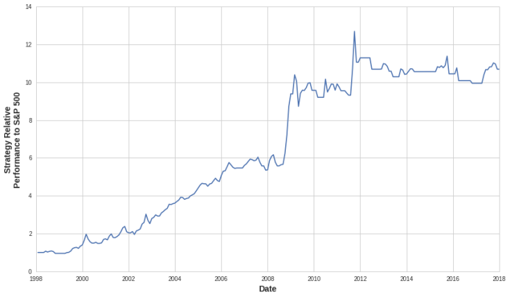
Here’s a breakdown of the periods of performance relative to the S&P 500:

• In the late 90s, the strategy is in global small-cap stocks more often than the S&P 500 which allowed it to slowly pull ahead.
• In the early 2000s, the strategy was largely in treasuries while stocks were losing money – further advancing the strategy’s lead over the benchmark.
• In the mid-2000s, the strategy stayed with small-cap global stocks which did quite a bit better than US stocks.
• In 2008 the strategy was mostly in treasuries which contributed to a large outperformance relative to the market/benchmark.
• In 2009, 2010, and 2011 it was mostly in small-cap global but it’d didn’t have much different performance relative to the S&P 500 – so no loss or gain.
• In late 2011, it got back into treasuries which went up while stocks went down.
• Since then it has largely been in the S&P 500 so no loss or gain has been made.

And that’s the key – with the benchmark being one of our three options – we ride it when it’s doing well thus minimizing the chance of prolonged tracking error leading to losses.  This is also exactly why I wanted such a strategy, the US stock market has done unusually well over the last 9 years.  I’m happy to have ridden most of that but I needed to find a way to emotionlessly allocate my money to ex-US stocks and bonds if/when necessary.  At this stage, I’m looking for tracking error… I just need an algorithm to make the decisions for me.

Concerns

Let’s try and poke some holes in the strategy and discuss why some of these concerns aren’t a big deal, and why some may be justified:

• Not Enough Assets
• Treasuries in a Rising Rate Environment?!
• Too Much Work
• Cost and Taxes
• Overfit
• International Explorer Fund is an Active Fund…
• Market Timing Never Works
• Daily Volatility

Not Enough Assets

Are three assets enough?  I think these three are diverse and uncorrelated enough to say yes.

But I still wanted to get some of my favorite assets in the strategy like consumer staples, mid-cap value, and emerging markets.  Consumer staples actually works pretty well in the strategy, in fact, it’s a little better to include it – here’s the link to the performance with it in. But it will require more changes and a higher tracking error.

I thought we could pair mid-cap value with S&P 500 to find the US asset that’s doing better then pair the better one against the ex-US asset.  This approach seems to work pretty well when using the 3, 6, and 12 month returns instead of 1, 3, and 6.  Use this same logic to pair small cap ex-US against emerging markets which also works well. This “dual squared” strategy seems to work when tested in Quantopian but it’s a bit too complicated to test in Portfolio Visualizer… and this is probably not a good sign.  I want something simple that I can stick with.  I also want to minimize my tracking error and the increased options that aren’t the S&P 500 will increase the tracking error.

Treasuries in a Rising Rate Environment?!?

Treasury yields have been dropping since 1981 which means we have witnessed the greatest bond bull market in history (as rates drop, prices increase). Below is a plot of rates over time compared to the real return on your investment (taking into account the change in bond pricing as well as inflation).  Up until early 1980s bonds didn’t offer very exciting real returns.  But from that point on – watch out!  Rates dropped from historic levels and your returns would have gone up accordingly.  Now rates should head upward which may lead to negative real returns moving forward.

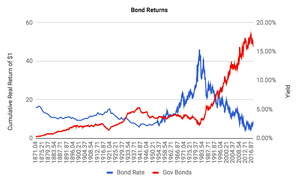
But I look at this plot and see the choppiness that occurred over the last 50 years.  Yes, rates have largely been dropping for 30 years but there were times it quickly dropped (and later rebounded) – and it is these accelerated moves that we’re trying to capture.  And even in the 1970s when bonds were largely losing money, there were still times they were moving the other way, ideally, during times stocks were doing poorly.

The strategy is not telling you to buy and hold long-term Treasuries on their own but instead, buy them when stocks are heading down.  Then sell them when/if stocks start recovering.  We’re only trying to take advantage of the swings.

That being said… I still am nervous about long-term Treasuries.  So you could consider playing treasuries against TIPS, specifically just looking at the trailing 1-month return between the two to decide.  This simple strategy has also done well, but it will require more switching due to the short look-back period.

Too Much Work

It may seem like there is a lot of switching between assets and therefore it’s a lot of work.  But that isn’t entirely true.  The average holding time is over 4 months which means most months you will be doing nothing.  And even when there is a change it’s buying & selling one asset.  If you are in a 401k it is one rebalance screen – literally takes less than a minute, per month.  I’m good with that.  I’ll also give the tools to let you make the calculations in seconds with Quantopian. Portfolio Visualizer seems to update pretty quickly too.  This link will always give most up-to-date information.  When I checked on April 1st 2018, Portfolio Visualizer had already indicated that small-cap ex-US is the asset to be in.

Cost and Taxes

This strategy works best for retirement accounts where taxes don’t matter.  These accounts should typically not have any rebalancing fees.  IRAs with major brokerages have commission-free ETFs too.  Even with fees, there are relatively few transactions so they become pretty insignificant.  Using Quantopian and Interactive Brokers’ fees with a $10,000 initial investment in 2004 the final balance in mid-March 2018 was $61,451 with no fees, $61,397 with fees.

If you are interested in using this in a Robinhood account that is taxable – you benefit from again no fees.  But you will have taxes to deal with.  The tax drag is still less than the historical outperformance.

Overfit Strategy

One of the concerns of “quants” and backtests is that all we did was find a strategy that worked well in the past due to some anomaly that has no chance of repeating again in the future.  I was cognizant of this risk when looking into the strategy which is helped define the simplicity of it.  An overly complex strategy with arbitrary signal ratios would be more suspect.  The relative momentum between the assets also helps in this regard.

Another way we fought the risk of overfitting was with the inclusion of multiple timing periods. Here’s a review of the performance for a $10,000 investment in January 1998 to March 2018:

• $39,063 for S&P 500
• $136,993 for only looking at 12-month relative momentum signal
• $251,954 for 6-month signal
• $282,374 for 3-month signal
• $403,440 for 1-month signal (but 149 timing periods)
• $425,417 for 1 + 3 + 6 month score (with “only” 60 periods)

A final fight against the risk of overfitting is if the strategy makes logical sense.  Although I find momentum to be a “stupid” factor (I’d prefer a more value-based one… maybe the combination of the two is best!? – the topic of a future post) it makes sense.  And the fact you can wrap your head around why its working is important – it can’t be only logical to a machine.  Although there are more and more machine-generated trades – the market is still full of human participants.  And people like chasing the asset that’s doing well.  We’ll ride that wave until a better one comes along.

International Explorer Fund is an Active Fund

The Vanguard International Explorer fund (VINEX) is the oldest (1997) and the least expensive (0.38%) small-cap international fund I could find which is why it was used in the long backtests.  But a look at the portfolio characteristics compared to Vanguard’s ex-US small-cap ETF (VSS) (started in 2009 with a 0.13% expense ratio) highlights that there are some deviations between the active fund and the index.  So did we get lucky?

VINEX’s portfolio is more mid growth compared to VSS’s portfolio which is evenly distributed between mid/small and growth/value.  They also have a different sector breakdown with currently more industrials and less defensive sectors.  But it’s an active fund so it’s moved around quite a bit over the years and maybe our strategy’s performance was due to the historically great performance that the VINEX management team provided – which may not repeat itself?

So let’s find another small-cap ex-US stock fund with a long history to drop into the strategy and see how it does.  The Oppenheimer International Small-Mid fund (OSMAX) was launched in 1997.  Comparing the results using VINEX to OSMAX from 1999 to March 2018 with a $10,000 initial investment:

• $30,371 for S&P 500
• $346,958 with VINEX
• $566,100 with OSMAX

Holy smokes, maybe I should have used the Oppenheimer fund in my original post!?  I think this gives some credence to the strategy overall, but now I’m curious why the Oppenheimer fund worked quite a bit better?

Comparing the performance of OSMAX, VINEX, and VFINX (S&P 500) in Morningstar shows that the two international funds track each other fairly well although they have noticeable periods of divergence.

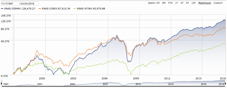
A look at the portfolio of OSMAX shows that it is even more heavily in mid-cap growth than VINEX which may suggest that that asset works better.  Or it’s just complete luck that it works better than VINEX and it may be overfitting to suggest that fund.  I think we’re better off saying the index of small-cap ex-US stocks does well in the strategy and that seemingly any fund in that index would have also done well.

Market Timing

The market returned 7.7% annually from 1997 through 2016, but if just the 10 best days were missed – the annual return dropped to 4.4%.

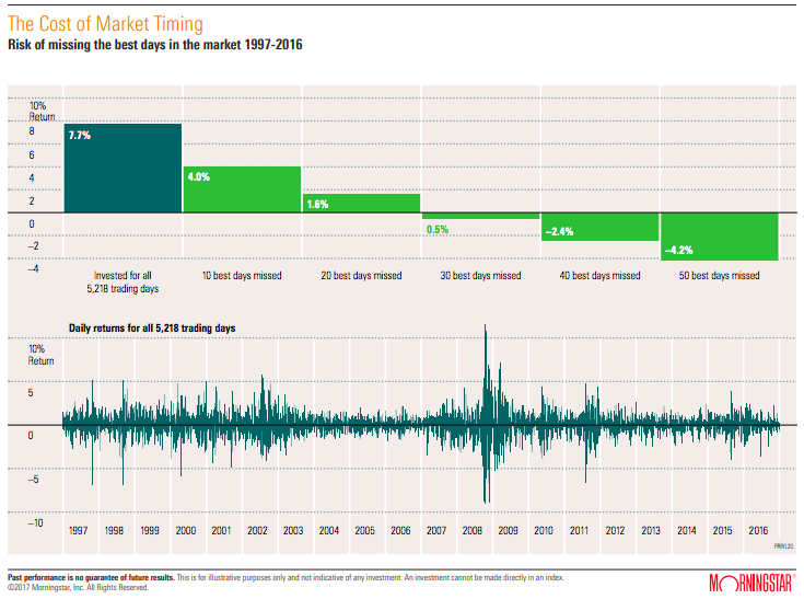
A $10,000 investment over 10 years with a 7.7% annualized return works out to $21,000.  If you missed just 10 days that came to $14,800.  Missing just a few good days can have a significant impact on performance which is why trying to time these days is particularly risky.

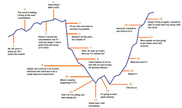
There are many posts out there that discuss why market timing is a fools game.  One from Schwab discusses how even picking the best month each year is barely better than just investing at the start. This one from ValueWalk has a particularly funny image I’ve posted below.

But the pitfalls of why market timing doesn’t work is exactly why… I want to utilize a market timing strategy and play the fools game!  Market timing doesn’t work because you’re trying to predict the future and you’re trying to make a judgment call based often on emotion.  Emotion and investing don’t mix well – but deliberate rules may help overcome the difficulties of market timing to follow the trends.

The other point I’d like to make is that we’re not necessarily trying to have our market timing strategy pick the best asset right every time (of which we only have a 33% chance) – instead, it’s more important to not pick the worst asset (a 67% chance).  The key to long-term gains is compounding the gains which are exponentially helped by minimizing the losses.  This strategy won’t prevent you from avoiding a sudden drop, but it pulls out of the prolonged declines.

Daily Volatility

The final risk of this strategy is the risk of the assets we’ll be tasked with holding.  Although they are fairly diversified on their own and they work well in concert with the other two assets over the long haul, on a day-to-day basis there can be quite a lot of volatility.  This is especially topical in today’s investment environment.  With a president who chooses to govern via Twitter posts, we are susceptible to very volatile days.  And when we’re only in one asset we’ll be forced to ride with that volatility.  This strategy is not a hedge fund trying to minimize volatility – its main task is to maximize returns.

This may be why you choose (and I’d recommend) to use this strategy as part of your overall investment portfolio – not the entirety of it.  Add some other assets that you’ll keep fixed such as gold, TIPS, mid-cap value, consumer staples, and emerging markets for example. Then in the remaining portion of your portfolio that you feel comfortable with, adopt this momentum strategy.  That way you can benefit from some of the long-term potential opportunity this strategy presents without being subjected fully to the day-to-day volatility… unless of course you are fully aware of it and want it. Get some!

---

Show Me More Data!

I was ready to publish this post about a month before I finally did.  This was largely due to the fact I didn’t feel comfortable publishing such a strategy without doing a more stringent analysis on how it has performed.  I needed monthly data going back over 100 years!  Thankfully Robert Shiller publically posts data going back to 1871 that I found. I compiled this data, added in MSCI index data, cleaned it a bit, and calculated the momentum signals in this google doc.

I was a bit nervous to find the data to then do the calculations and realize that my backtest on the last 20 years was an anomaly.  The true test of a quantitative strategy is if it does well in out-of-sample testing.  But another effective way to see if it has been overfitted is to try it on data not seen before.  And now I had an extra 120 years of data… how did it do?

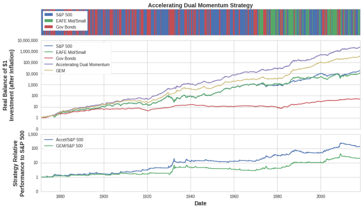
I was extremely relieved but even more excited to find that the accelerating momentum signal had worked very well going all the way back to 1871!  An investment in this strategy would have produced over 100x more return than an investment in the S&P 500 over that time.

A few caveats regarding this longer dataset to the more recent 20 years:

• Much of the historical data doesn’t have global equities.  They first enter the scene in 1970 but EAFE small/mid doesn’t start until 1994.  So I used EAFE large for 1970 to 1994 and ignored international equities the rest of the time – it was just US stocks vs US government bonds
• Bonds are only looking at the 10-year yield.  We found that long-term treasuries swing harder so theoretically they would further improve the long-term performance but I couldn’t find that data.  I also had to assume the yield curve was flat to calculate bond pricing.
• Again no taxes or fees – but this shouldn’t be a big deal for a monthly strategy that is used in a retirement account

Some tidbits of summary from the historical data that deserves its own future post (this one is already getting quite long!):

• Annual real (after inflation) returns:
  • 10.5% – Accelerating Dual Momentum (ADM)
  • 9.1% – GEM
  • 6.9% – S&P 500
  • 2.7% – Bonds
• Maximum drawdown (after inflation):
  • -34% – Accelerating Dual Momentum (ADM)
  • -43% – GEM
  • -77% – S&P 500
  • -57% – Bonds
• Worst 1-year loss (after inflation):
  • -21% – Accelerating Dual Momentum (ADM)
  • -33% – GEM
  • -58% – S&P 500
  • -22% – Bonds

The bond drawdown of 57% is surprising… but the performance of the accelerating dual momentum strategy is very encouraging!  Another way to measure risk is to plot the trailing 30-year return to see how the strategy does in any given investment period.

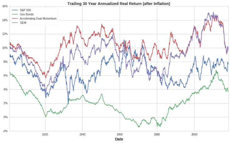
Accelerating dual momentum beats the S&P 500 in virtually every 30 year period except the 30 years immediately following the great depression.  Now the strategy may have lost relative to the S&P 500 over that time but only performed marginally lower and did so after just avoiding much of the carnage of the great depression (and some other bumps between then and 1963).

What Happens Next?

Who knows?  I certainly don’t.  And that’s the point.  I’m going to follow the trend with hope that it can help me avoid prolonged downturns and maximize accelerating upward swings – but there’s no guarantee that the strategy won’t do the exact opposite.

---

How to “Live Trade” the Strategy?

Portfolio Visualizer

You can use this link to check monthly at Portfolio Visualizer which asset you should be in.  Go to the timing periods tab and scroll all the way to the bottom.  This updates daily.  Then you can make the switch in whatever account you’re doing this in manually.  Should take all of 5 minutes a month.

Quantopian

You can check out my post on Quantopian where I provide the source code of an algorithm that will “live paper trade” the strategy.  Again you’d have to check back monthly but you’d have some added ability to customize as you see fit.  A caveat between this and the portfolio visualizer method, however, is that in portfolio visualizer it uses total returns with dividends.  It also takes into account the length of the month.  In Quantopian I’m looking back a fixed number of days.

Engineered Portfolio Service

Last but not least – Chris and I can get off our butts and make a real service out of all this analysis.  To start we can email those interested monthly to provide the update on what to do (I’m doing this already for a few friends, doesn’t take any more work to add recipients!).

Longer term though we envision a software service that will connect directly to your Robinhood investment account to do the trades for you.  We’d have to charge a nominal amount for this, maybe $10 a month.  I can do the monthly email for free though.  Sign up by clicking the link/image below and filling out the form for those emails and to get notified once we finally build out that software service.

The author(s) of this site have no formal financial investing training or certifications.  The content on this site is provided as general information only and should not be taken as investment advice. All site content shall not be construed as a recommendation to buy or sell any security or financial instrument, or to participate in any particular trading or investment strategy. The ideas expressed on this site are solely the opinions of the author(s) and do not necessarily represent the opinions of sponsors or firms affiliated with the author(s). The author may or may not have a position in any company or advertiser referenced above. Any action that you take as a result of information, analysis, or advertisement on this site is ultimately your responsibility. Consult your investment adviser before making any investment decisions. This site/blog contains the current opinions of the author; the author’s opinions are subject to change without notice. This site is for informational purposes only and should not be considered as investment advice or a recommendation of any particular security, strategy or investment product. The charts and comments are only the author’s view of market activity and aren’t recommendations to buy or sell any security. Market sectors and related ETFs are selected based on his opinion as to their importance in providing the viewer a comprehensive summary of market conditions for the featured period. Chart annotations aren’t predictive of any future market action rather they only demonstrate the author’s opinion as to a range of possibilities going forward. All material presented herein is believed to be reliable but we cannot attest to its accuracy. The information contained herein (including historical prices or values) has been obtained from sources that Engineered Portfolio considers to be reliable; however, Engineered Portfolio makes no representation as to, or accepts any responsibility or liability for, the accuracy or completeness of the information contained herein or any decision made or action taken by you or any third party in reliance upon the data. Some results are derived using historical estimations from available data. Investment recommendations may change and readers are urged to check with tax advisors before making any investment decisions. Opinions expressed in these reports may change without prior notice. This memorandum is based on information available to the public. No representation is made that it is accurate or complete. This memorandum is not an offer to buy or sell or a solicitation of an offer to buy or sell the securities mentioned. The investments discussed on this site/blog may be unsuitable for investors depending on their specific investment objectives and financial position. Past performance is not necessarily a guide to future performance. The price or value of the investments to which this report relates, either directly or indirectly, may fall or rise against the interest of investors. All prices and yields contained in this report are subject to change without notice. This information is based on hypothetical assumptions and is intended for illustrative purposes only. PAST PERFORMANCE DOES NOT GUARANTEE FUTURE RESULTS.